How large-scale systems check username availability in milliseconds
The Bloom filter trick that helps avoid millions of unnecessary database queries.
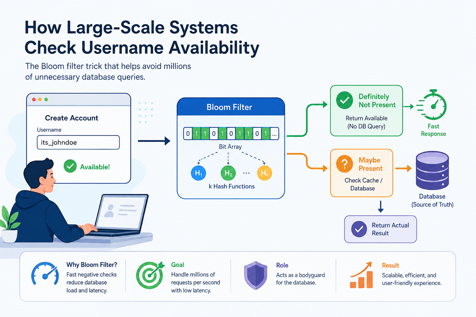
A simplified request flow showing how Bloom Filters reduce database load in large-scale systems.
Imagine you’re signing up for Gmail. You type:
its_johndoe
…and almost instantly:
✔ Available
No spinner. No awkward pause. Just an answer.
At the scale of services like Gmail, that tiny green checkmark hides a brutal reality: there are billions of usernames , massive sign‑up traffic , and strict latency budgets . The real systems question isn’t:
“How do we query fast?”
It’s:
“How do we avoid querying at all for most requests?”
A Bloom filter is one of the cleanest answers.
We’ll cover:
- The deceptively hard question
- The obvious approaches (and why they hurt)
- The key insight: ask a cheaper question first
- Enter the Bloom filter (the database’s bodyguard)
- How a Bloom filter works (intuition first)
- The math (why “maybe” happens)
- Implementation (a clean Python baseline)
- Hashing in production: what real systems do instead
- How large-scale systems use Bloom Filters
- Sizing it: a real example (where people get stuck)
- Operational realities (the stuff that often gets skipped)
- Limitations (so you don’t overuse them)
- Conclusion
- Further Reading
1) The deceptively hard question
Design a username‑availability checker for a Gmail-like service.
Requirements:
- 1B+ usernames already taken
- Capable of handling millions of requests/second (at peak global traffic)
- Strict latency (tens of milliseconds)
- High availability (must survive spikes)
Every request asks the same thing:
Is this username already taken?
Your enemies are: network hops , disk I/O , and doing the same expensive work millions of times .
2) The obvious approaches (and why they hurt)
Option A: scan the whole list (don’t do this)
Linear search:
O(n)
For a billion entries, this is dead on arrival.
Option B: query the database (better, still expensive)
SELECT 1 FROM users WHERE username = 'its_johndoe';
Even with indexes, each query still implies:
- a network hop
- CPU work
- cache misses
- index traversal
- contention under concurrency
It works. But doing it millions of times per second gets costly fast.
Option C: indexed lookup (fast, not free)
B+ trees (or similar indexes) give:
O(log n)
But “log n” still means real work . And if you miss hot caches, that work becomes visible to users.
3) The key insight: ask a cheaper question first
Instead of immediately asking the database:
“Does this username exist?”
…ask a cheaper question first:
“Is this username definitely NOT present?”
Because the fastest database query is often the one you never have to execute.
This is the Bloom filter mindset:
- fast negative checks
- rare expensive confirmations
4) Enter the Bloom filter (the database’s bodyguard)
A Bloom filter is a probabilistic data structure for membership queries with two possible answers:
- Definitely not present (100% certain)
- Maybe present (needs confirmation)
So it doesn’t replace the database. It protects it.
A typical production flow:
              Request
                 ↓
            Bloom Filter
          ↙              ↘
Definitely Not         Maybe Present
    Present                  ↓
       ↓              Check Cache/Database
       ↓                     ↓
Return immediately     Return Actual Result
If the Bloom filter says “definitely no”, you can immediately return Available .
If it says “maybe”, you fall back to your source of truth.
5) How a Bloom filter works (intuition first)
A Bloom filter is basically:
- a bit array (a long sequence of 0s and 1s)
- k hash functions
Step 1: start with all zeros
[0 0 0 0 0 0 0 0 0 0]
Step 2: insert a username
Insert "john_doe".
Compute k positions using hashes:
h1(john_doe) → 1
h2(john_doe) → 5
h3(john_doe) → 7
h4(john_doe) → 11
Flip those bits to 1:
[0 1 0 0 0 1 0 1 0 0 0 1]
Step 3: insert another username
Insert "john_doe123":
h1(john_doe123) → 2
h2(john_doe123) → 5
h3(john_doe123) → 8
h4(john_doe123) → 10
Now:
[0 1 1 0 0 1 0 1 1 0 1 1]
Step 4: query
To query "its_johndoe", compute the same k positions.
- If any required bit is 0 → definitely not present
- If all are 1 → maybe present
Key idea: we’re not storing usernames — we’re storing hash fingerprints that can overlap.
That overlap is exactly why Bloom filters can have false positives .
6) The math (why “maybe” happens)
Let:
- m = number of bits in the array
- n = inserted elements
- k = number of hash functions
After inserting n items, the probability a bit is still 0 is approximately:
P(bit = 0) ≈ e^(-kn/m)
So the probability it’s 1 is:
P(bit = 1) = 1 - e^(-kn/m)
A false positive happens when all k checked bits are 1:
P(false positive) = (1 - e^(-kn/m))^k
What this means in plain English
- Larger m (more bits) → fewer collisions → fewer false positives
- More k hashes → better discrimination up to a point
- Larger n (more items) → the filter gets “fuller” → more false positives
There’s also an optimal k that minimizes false positives:
k = (m/n) * ln(2)
7) Implementation (a clean Python baseline)
Here’s a minimal Bloom filter (with sizing formulas):
import math
import hashlib

class BloomFilter:
    def __init__(self, expected_elements: int, acceptable_fp_perc: float):
        # Calculations
        n = expected_elements
        fp = acceptable_fp_perc
        m = int(-(n * math.log(fp)) / (math.log(2) ** 2))
        k = int((m / n) * math.log(2))

        # Assignment
        self.M = m
        self.K = k
        self.bits = [0] * m

    def _hashes(self, data: str):
        # base hashes (double hashing)
        h1 = int(hashlib.sha1(data.encode()).hexdigest(), 16)
        h2 = int(hashlib.sha256((data + "salt").encode()).hexdigest(), 16)
        M, K = self.M, self.K # Alias
        for i in range(K):
            yield (h1 + i * h2) % M

    def add(self, data: str):
        for idx in self._hashes(data):
            self.bits[idx] = 1

    def exists(self, data: str) -> bool:
        for idx in self._hashes(data):
            if self.bits[idx] == 0:
                return False
        return True
Note: This implementation is intentionally kept simple to demonstrate how Bloom filters work. In production, you wouldn’t typically use cryptographic hash functions like
SHA-256. While they're stable and correct, they're much slower than non-cryptographic alternatives and provide security guarantees that Bloom filters don't require.
8) Hashing in production: what real systems do instead
At first glance, hashlib.sha256() or Python’s built‑in hash() may look convenient, but they’re not ideal for Bloom filters at scale.
Why not use Python’s built‑in hash()?
Python’s built‑in hash is not stable across runs by design:
hash("john") → 12345   (run 1)
hash("john") → 98765   (run 2)
This breaks Bloom filters because the same input must always map to the same bit positions.
Why not use cryptographic hashes?
Using sha256, sha1, etc. is correct but inefficient:
- too slow for high throughput
- unnecessary cryptographic guarantees
- excessive CPU cost per lookup/insertion
What production systems use instead
Real‑world systems prefer fast, non‑cryptographic hashes:
- MurmurHash
- FNV‑1a
- xxHash
They provide:
- high speed
- good distribution
- deterministic output
Double hashing (Kirsch–Mitzenmacher optimization)
Instead of computing k separate hashes, production systems use a trick:
h1 = hash1(x)
h2 = hash2(x)

index(i) = (h1 + i * h2) % m
This generates k hash values using only two base hash computations — much faster while maintaining good distribution properties.
9)How large-scale systems use Bloom Filters
A realistic flow usually isn’t just “Bloom filter → DB”. It’s layered:
Client
  ↓
 API
  ↓
Bloom filter (Fast negative check)
  ↓
Cache (Redis / Memcached)
  ↓
Database (source of truth)
Why add cache if you already have a Bloom filter?
Because Bloom filters don’t answer “yes” with certainty.
- A Bloom filter is great at rejecting negatives
- Cache is great at serving hot positives (popular usernames, retries, bots)
- DB is final truth
Where does the Bloom filter live?
Typical choices:
- in‑process memory (fastest per request)
- shared in‑memory service (easier updates, slightly more latency)
- embedded in storage layer (e.g., RocksDB tables)
At extreme scale, you may shard Bloom filters by prefix or hash range.
10) Sizing it: a real example (where people get stuck)
Say you want:
- n = 1,000,000,000 usernames (1B)
- false positive rate p = 1% (0.01)
The standard sizing formula for bits ( m ) is:
m = - (n * ln(p)) / (ln(2)^2)
For p = 0.01:
- ln(0.01) ≈ −4.6052
- ln(2)² ≈ 0.48045
So:
m ≈ 9.6 * n bits
That’s roughly:
- m ≈ 9.6 billion bits
- ≈ 1.2 billion bytes
- ≈ ~1.2 GB
And the optimal k :
k = (m/n) * ln(2) ≈ 9.6 * 0.693 ≈ 6.65
So k ≈ 7 hash functions .
Interpretation
To get ~1% false positives for 1B items, you might spend ~1.2GB of memory per filter.
That sounds big — until you compare it to the cost of hammering a database with millions of unnecessary queries.
Practical trick
Many systems don’t keep one global 1.2GB filter per node. They:
- shard the filter
- compress or use cache‑friendly bitsets
- keep one per region/cluster
- use a smaller n for “active usernames” and fall back for cold data
11) Operational realities (the stuff that often gets skipped)
Bloom filters are not “set and forget”. In real systems you must think about:
1) Refresh / rebuild strategy
Usernames change.
- New signups add items
- Deletions are rare for usernames, but may exist
Classic Bloom filters don’t support deletion, so systems typically:
- rebuild periodically (daily/weekly)
- rebuild when false‑positive rate crosses a threshold
- maintain a small “delta filter” for recent inserts
2) Measuring false positives in production
You can estimate false positives by tracking:
- Bloom filter says “maybe”
- DB says “not found”
That’s a false positive event. Monitoring this ratio tells you when the filter is too full.
3) Failure modes
If the Bloom filter is missing/unavailable, degrade gracefully:
- fall back to cache/DB
- accept higher latency, but preserve correctness
Bloom filters are an optimization layer — not correctness infrastructure.
12) Limitations (so you don’t overuse them)
Bloom filters are amazing, but:
- false positives are possible (never false negatives)
- deletion is not supported (unless you use variants)
- parameter tuning matters (m, k, n)
Common alternatives:
- Counting Bloom Filter (supports deletes)
- Cuckoo Filter (good for deletes, often competitive)
- XOR Filter (very memory‑efficient for static sets)
13) Conclusion: the best optimization is skipping the work
Bloom filters feel almost magical the first time you “get” them:
- they don’t store the data
- they don’t promise certainty
- and yet they can make systems dramatically faster
Because the principle underneath is pure engineering gold:
Avoid expensive work whenever you can — don’t just optimize it after you’ve already committed to doing it.
So the next time Gmail instantly says a username is available, picture a tiny bit array whispering:
“Nope — don’t even bother the database.”
14) Further Reading
If you’d like to explore Bloom filters in more depth, these are excellent resources:
- Burton H. Bloom (1970). Space/Time Trade-offs in Hash Coding with Allowable Errors.
- Adam Kirsch & Michael Mitzenmacher (2006). Less Hashing, Same Performance: Building a Better Bloom Filter.
- **Designing Data-Intensive Applications ** — Chapter on storage engines and probabilistic data structures.
- Redis documentation on probabilistic data structures (Bloom filters, Cuckoo filters, HyperLogLog).
- Apache Cassandra documentation on Bloom filters in SSTables.